
The basics of slug flow, Calculation of Slug forces, and static analysis methodology in Caesar II are provided in my last article titled “Static Analysis of Slug Flow”. Click here to read the same. In this article, We will explain the methods for performing the slug flow analysis using the Dynamic Spectrum Method of Caesar II Software.
Reason for Dynamic Slug Flow Analysis of Piping System?
The system responses are very much different with respect to dynamic slug loads as compared to a static load of the same magnitude. As static load is applied slowly, the piping system gets enough time to internally distribute the loads and react, resolving the forces and moments and keeping the system in equilibrium. Hence, the pipe movement is not visible.
On the other hand, a dynamic slug load quickly varies with respect to time and hence the piping system does not get sufficient time to distribute and resolve the forces. This results in an unbalanced slug force that leads to pipe movement. So it’s always preferable to perform dynamic analysis when dynamic loads are involved to get real analysis results.
Dynamic Slug Flow Module of Caesar II
For performing dynamic slug flow analysis, Caesar II software provides a very nice module, dynamic analysis module where we have to simply provide the input parameters to get the output result. In the following paragraphs, we will learn the steps for performing Dynamic Slug Flow using Water Hammer/ Slug Flow (Spectrum) method.
Before you start the dynamic slug flow analysis you have to perform a conventional static analysis of the system (without using any slug force) and qualify the system from all stress criteria (Thermal, Sustained, Occasional, as applicable).
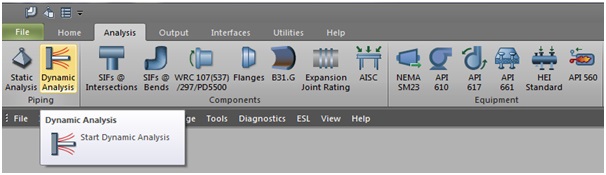
To open the dynamic module in Caesar II click on the dynamic analysis button as shown in Fig.1.
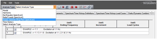
When you click on the dynamic analysis button following window (Fig.2) will open. Select Slug Flow (Spectrum) from the drop-down menu. The window will be filled with some pre-existing data. For clarity simply select all those and delete them. Now we have to provide inputs for analysis.
During dynamic slug flow analysis, our first input will be the generation of a response spectrum profile. Slug load is one type of impulse load. So the magnitude of the load varies from zero to some maximum value, remains constant for a time, and then reduces to zero again. The force profile can be represented by a curve as shown in Fig. 3.
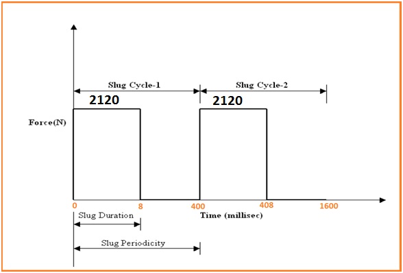
So from the above profile, it is clear that in addition to the slug force (Refer to Static method of Slug Flow using Caesar II for calculation of slug force), we need to calculate two additional parameters, a) Slug Duration and b) Slug Periodicity.
Slug Duration
Slug duration is defined as the time required for the slug to cross the elbow. Mathematically it can be denoted as, Slug Duration=Length of Liquid Slug/Velocity of Flow.
Slug Periodicity
Slug Periodicity can be defined as the time interval for two consecutive slugs hitting the same elbow. So mathematically it can be denoted as Slug Periodicity = (Length of Liquid Slug + Length of Gas Slug)/Velocity of Flow.
Generating Spectrum Profile for Slug Flow
Let’s assume that the calculated slug duration is 8 milliseconds and periodicity is 400 milliseconds as shown in Fig. 3. We will use these data for the generation of spectrum profiles.
Now Refer to Fig. 4 and input the data as mentioned below:
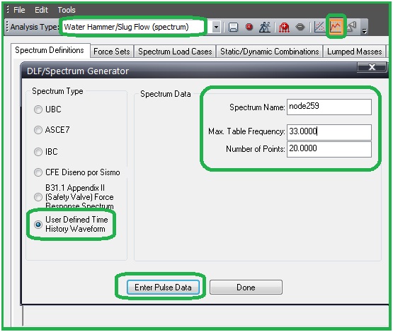
When you click on Enter Pulse data it will open the window where we have to enter the data for spectrum profile generation. From the above curve at time 0 the force is 2120 N the same force will be active for the next 8 milliseconds till the slug crosses the elbow. Then at time, 8.1 millisecond forces will be reduced to zero. And the same zero force will be there till 400 milliseconds. Then the next cycle will start. i.e., at time 400.1 milliseconds, the force will be again 2120 N. That way enter data for at least two cycles as shown in Fig. 5:
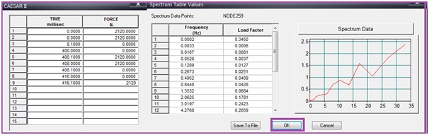
Clicking the Save / Continue button will convert the time history into its equivalent force response spectrum in terms of Dynamic Load Factor versus Frequency and the screen “Spectrum Table Values “as shown in Fig. 5 will appear.
Be sure to specify a unique spectrum name, as this processor will overwrite any existing files of the same name.
By clicking OK, the processor will load the appropriate data in the Spectrum Definitions tab in Dynamic Input and move the data to the Dynamic Input.
Once the spectrum profile is generated click on the force sets button and enter the slug force with the proper direction in the fields as shown in Fig. 6:
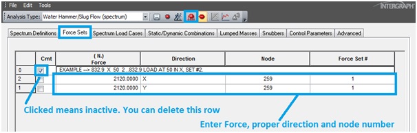
- Click on the + button to add more rows and the – buttons to delete rows.
- In the force set field, input a numeric ID which will be used to construct dynamic load cases.
Creating Dynamic Slug Flow Load Cases for Analysis
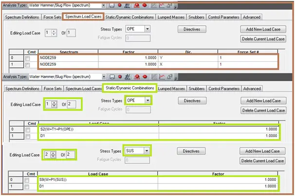
After that, click on the Spectrum load cases menu and create the required load cases for dynamic analysis. You have to specify at least two load cases as shown.
- Operating + Dynamic for nozzle and support load checking.
- Sustained + Dynamic for stress checking.
Refer to Fig. 7 for load case preparation
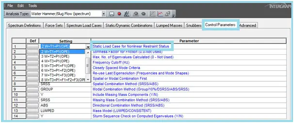
Finally, click on the control parameters button and select the load case for which you want to perform the analysis. Normally operating load case is selected (Refer to Fig. 8) for dynamic analysis. Keep all other parameters as it is. Now click on batch run to obtain the analysis results. Fig 9 shows typical analysis results.
Output Results from Dynamic Slug Flow Analysis
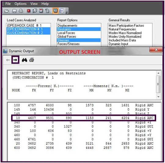
- Fig. 9 shows a typical output screen for dynamic slug flow analysis in Caesar II.
- The highlighted node 10 is for the nozzle.
- All support and nozzle loads are to be checked.
- Stresses are to be kept below code allowable values.
- The highlighted direction sign will show other load case combinations.
Some Important Points to Consider
- Piping vibration due to any two-phase flow can be reduced/arrested by proper support of the piping system. Normally following supports are used:
- HOLD DOWN SUPPORTS WITH 0 GAP
- GUIDE SUPPORTS WITH 0 GAP
- AXIAL STOPS WITH 0 GAP
Whenever modifying any support perform static analysis and keep the system stresses within the allowable limit.
- Sometimes vibration-absorbing material (like PTFE) is used to reduce the transfer of vibration to connected systems.
- It is preferred to keep the natural frequency of the piping system above 4 Hz for Vibration-prone lines.
- The formation of Slug Flow can be reduced by
- By reducing line sizes to a minimum permitted by available pressure differentials.
- By using a low-point effluent drain or bypass.
- By arranging the pipe configurations to protect against slug flow. E.g. in a pocketed line where liquid can collect, slug flow might develop. Hence pocket is to be avoided.
- By Installing a Slug Catcher
Online Course on Dynamic Slug Flow Analysis
If you still have doubts, then the following online course is just perfect for you:
Some handpicked useful resources for you…
Static Analysis of Slug flow
How to Model Slug Flow Loads
An Introduction to Pressure Surge Analysis
Understanding Centrifugal Compressor Surge and Control
Load Cases for Stress Analysis of a Critical Piping System Using Caesar II
Water Hammer Basics in Pumps for beginners
Pipe Stress Analysis from Water Hammer Loads
Very welll explained. Thanks.
How to get length of liquid slug & gas slug for slug duration and Periodicity calculation?
For Hands on Practise ……Please post input DATA of example ALSO , in form pictures of iso’s, pids ect
Sir Please provide with System Isometrics P& Id deimensions and pressure temp, mat data with code ASME…..material, so that a learner solve it easily and acheive his goals by getting results shown in your blog
Nice Blog keep growing …ALL THE BEST.
Thanks for the article. Would like to see more dynamic analysis such as Time History, Harmonic analysis
How to get the length of liquid slug and gas slug ??
please confirm whether time history analysis is preffered over spectrum analysis for more accurate results
Hello, thank you for giving insight to this part of CII. I have one question and can’t find an answer anywhere. Why does my CII analysis for ISO 14692-2 (2017) give the message: “No code stress check processed” when I look at the Report Options: stresses.
Thank you, nice article.
I have one question, in the spectrum profile you used the force 2120 N, and in the Static Analysis you used the force DLF (2,0) * F which is 4240N for input into the model. So, please confirm that DLF is not intended for use in Dynamic Analysis, it is used only for Static Analysis of the piping system?
Again, thank you very much for all these explanations.
Yours sincerely,
Ivan
Your understanding is correct.